Python Figures

In [1]:

import nilearn as nl # nilearn for loading nifti
import os
import matplotlib.pyplot as plt
import matplotlib.ticker as ticker
import numpy as np
import nibabel as nib # nibable: loading nifti
from nilearn import plotting # nilearn plotting
from matplotlib.colors import ListedColormap # custom colormaps
import graphviz # graph
from PIL import Image # image resizing
import nilearn

In [2]:

figpath='/home/weberam2/Dropbox/AssistantProf_BCCHRI/Projects/Gavin_CSVO2/Quarto_Chisep_CSVO2_Manuscript/images/'

In [3]:

def apply_slice_cut_to_nifti(nii_gz_path, slice_cut):
    """
    Load a NIfTI image, apply a slice cut to extract a subregion, and return a new NIfTI image.

    Parameters:
    - nii_gz_path (str): Path to the input NIfTI (.nii.gz) file.
    - slice_cut (list): Slice cut specification in the form [slice_x, slice_y, slice_z].

    Returns:
    - nibabel.Nifti1Image: New NIfTI image object containing the extracted subregion.
    """
    # Load the NIfTI image
    nii_img = nib.load(nii_gz_path)
    nii_data = nii_img.get_fdata()

    # Extract the subregion using the slice cut
    slice_x, slice_y, slice_z = slice_cut
    subregion_data = nii_data[slice_x, slice_y, slice_z]

    # Create a new NIfTI image with the extracted subregion and original affine matrix
    subregion_img = nib.Nifti1Image(subregion_data, nii_img.affine)

    return subregion_img

In [4]:

basepath='/home/weberam2/Dropbox/AssistantProf_BCCHRI/Projects/Gavin_CSVO2/Data/'

In [5]:

slice_cut = [slice(60, 190), slice(50, 200), slice(None)]  # Define the slice cut [x, y, z]

In [6]:

nii_gz_relpath = 'QSM_SSS/qsm/sub-AMWCER18/mag_echo1.nii.gz'
nii_gz_path = basepath + nii_gz_relpath

mag = apply_slice_cut_to_nifti(nii_gz_path, slice_cut)

#plotting.plot_anat(anat_img=mag) #testing

In [7]:

nii_gz_relpath = 'QSM_SSS/calc_chi/sub-AMWCER18/STISuite_Last3Echos/S001_QSM_star.nii.gz'
nii_gz_path = basepath + nii_gz_relpath

qsm = apply_slice_cut_to_nifti(nii_gz_path, slice_cut)

In [8]:

nii_gz_relpath = 'Chi_sep/sub-AMWCER18/x_pos_SA_finalmask.nii'
nii_gz_path = basepath + nii_gz_relpath

parachi = apply_slice_cut_to_nifti(nii_gz_path, slice_cut)

In [24]:

cut_coords_qsm = (64,42,51)

# Set the number of rows and columns for the subplot grid
num_rows = 3
num_cols = 1

figsize=(10, 12)
fig = plt.figure(figsize=figsize)
gs = fig.add_gridspec(nrows=num_rows, ncols=num_cols, height_ratios=[1, 1, 1])
# Add subplots based on gridspec
ax1 = fig.add_subplot(gs[0,0])  # First subplot (top row)
ax2 = fig.add_subplot(gs[1,0])  # Second subplot (bottom row)
ax3 = fig.add_subplot(gs[2,0])  # Third subplot (bottom row, first column)

vmin, vmax = np.percentile(mag.get_fdata(), (2, 99.9))
plotting.plot_anat(anat_img=mag,
                      black_bg = False,
                      draw_cross=False, 
                      vmin=vmin, vmax=vmax, 
                      annotate=True, axes=ax1,
                  colorbar = False,
                  )

# Second plot (with colorbar for QSM)
plotting.plot_anat(
    anat_img=qsm,
    black_bg=False,
    draw_cross=False,
    vmin=-0.2, vmax=0.2,
    annotate=True, axes=ax2,
    colorbar=True,
    cut_coords=cut_coords_qsm,
)

plotting.plot_anat(anat_img=parachi,
                   black_bg = False,
                      draw_cross=False, 
                      vmin=0, vmax=0.2, 
                      annotate=True, axes=ax3,
                   colorbar= True,
                   cut_coords=cut_coords_qsm
                  )
fontsize=16
xoffset=-0.05
yoffset=1.05
# Add label "A" to the first subplot
ax1.text(xoffset, yoffset, 'A', transform=ax1.transAxes,
             fontsize=fontsize, fontweight='bold', va='top', ha='right')

ax2.text(xoffset, yoffset, 'B', transform=ax2.transAxes,
             fontsize=fontsize, fontweight='bold', va='top', ha='right')

ax3.text(xoffset, yoffset, 'C', transform=ax3.transAxes,
         fontsize=fontsize, fontweight='bold', va='top', ha='right') 

plt.figtext(.9, 0.37, r'$\chi$ (ppm)', ha='right', fontsize=11)
plt.figtext(.9, 0.098, r'$\chi$ (ppm)', ha='right', fontsize=11)

plt.savefig(figpath + "SampleImages.png", dpi=300, bbox_inches="tight")

plt.show()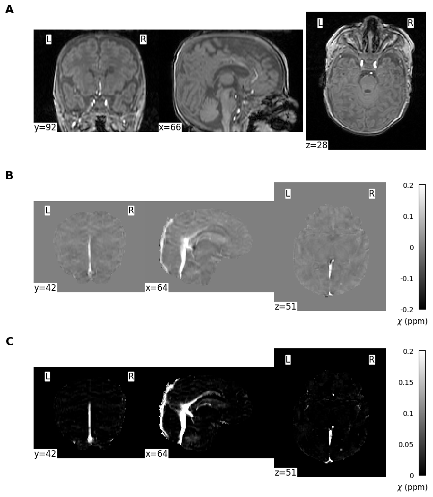

Figure 1: An example of subject imaging data. A sample coronal, sagittal, and axial slice is displayed for each image. (a) The 1st echo of the magnitude susceptibility weighted imaging sequence; (b) the final quantitative susceptibility mapping image; and (c) the paramagnetic component isolated from the quantitative susceptibility map. The color bars in (b) and (c) indicates the range of susceptibility \(\chi\) values in parts per million. y, x and z values represent the slice number in each plane (coronal, sagittal, and axial, respectively).

In [10]:

def plot_and_save_nifti_slice(nii_gz_path, slice_cut, single_slice_cut, figsize, out_path, cmap):
    """
    Load a NIfTI image, apply slice cuts, extract a single slice, plot the slice, and save as a PNG file.

    Parameters:
    - nii_gz_path (str): Path to the input NIfTI (.nii.gz) file.
    - slice_cut (list): Slice cut specification in the form [slice_x, slice_y, slice_z].
    - single_slice_cut (tuple): Single slice specification for extraction (e.g., [54, :, :]).
    - figsize (tuple): Figure size in inches (width, height).
    - mask_path (str): Path to save the PNG file.
    - cmap (str or matplotlib.colors.Colormap): Colormap for the plot.

    Returns:
    - str: Path to the saved PNG file.
    """
    # Load the NIfTI image
    nii_img = nib.load(nii_gz_path)
    nii_data = nii_img.get_fdata()

    # Apply slice cuts to extract a subregion
    if len(slice_cut) == 3:  # For 3D data [slice_x, slice_y, slice_z]
        subregion_data = nii_data[slice_cut[0], slice_cut[1], slice_cut[2]]
    elif len(slice_cut) == 4:  # For 4D data [slice_x, slice_y, slice_z, slice_t]
        subregion_data = nii_data[slice_cut[0], slice_cut[1], slice_cut[2], slice_cut[3]]

    # Extract a single slice
    single_slice_data = subregion_data[single_slice_cut]

    # Create a new figure with the specified figsize
    plt.figure(figsize=figsize)

    # Display the single slice with the specified colormap
    plt.imshow(single_slice_data.T, cmap=cmap, origin='lower')

    # Remove x-axis and y-axis ticks
    plt.xticks([])
    plt.yticks([])

    # Save the plot as a PNG file
    plt.savefig(out_path, dpi=300, bbox_inches="tight", pad_inches=0)

    # Show the plot (optional)
    plt.show()

    # Return the path to the saved PNG file
    return out_path

In [11]:

# nii_gz_relpath = 'QSM_SSS/calc_chi/sub-AMWCER18/STISuite_Last3Echos/mag_echo5.nii.gz'
# nii_gz_path = basepath + nii_gz_relpath

# magechofive_path="magecho5.png"
# out_path=figpath + initialmask_path

# plot_and_save_nifti_slice(nii_gz_path, slice_cut, single_slice_cut, figsize, out_path, cmap)

In [12]:

basepath

'/home/weberam2/Dropbox/AssistantProf_BCCHRI/Projects/Gavin_CSVO2/Data/'

In [13]:

nii_gz_relpath = 'QSM_SSS/calc_chi/sub-AMWCER18/STISuite_Last3Echos/mag_echo5.nii.gz'
nii_gz_path = basepath + nii_gz_relpath

single_slice_cut = (62, slice(None), slice(None))
figsize=(8, 8)
cmap= 'gray'

magechofive_path="magecho5.png"
out_path=figpath + magechofive_path

plot_and_save_nifti_slice(nii_gz_path, slice_cut, single_slice_cut, figsize, out_path, cmap)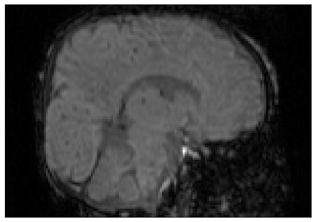

'/home/weberam2/Dropbox/AssistantProf_BCCHRI/Projects/Gavin_CSVO2/Quarto_Chisep_CSVO2_Manuscript/images/magecho5.png'

In [14]:

nii_gz_relpath = 'QSM_SSS/calc_chi/sub-AMWCER18/STISuite_Last3Echos/mag_echo5_sqr_brain_mask.nii.gz'
nii_gz_path = basepath + nii_gz_relpath

initialmask_path="InitialMask.png"
out_path=figpath + initialmask_path

plot_and_save_nifti_slice(nii_gz_path, slice_cut, single_slice_cut, figsize, out_path, cmap)

'/home/weberam2/Dropbox/AssistantProf_BCCHRI/Projects/Gavin_CSVO2/Quarto_Chisep_CSVO2_Manuscript/images/InitialMask.png'

In [15]:

nii_gz_relpath = 'QSM_SSS/calc_chi/sub-AMWCER18/STISuite_Last3Echos/dil7_echo5mask.nii.gz'
nii_gz_path = basepath + nii_gz_relpath

dilatedmask_path="DilatedMask.png"
out_path=figpath + dilatedmask_path

plot_and_save_nifti_slice(nii_gz_path, slice_cut, single_slice_cut, figsize, out_path, cmap)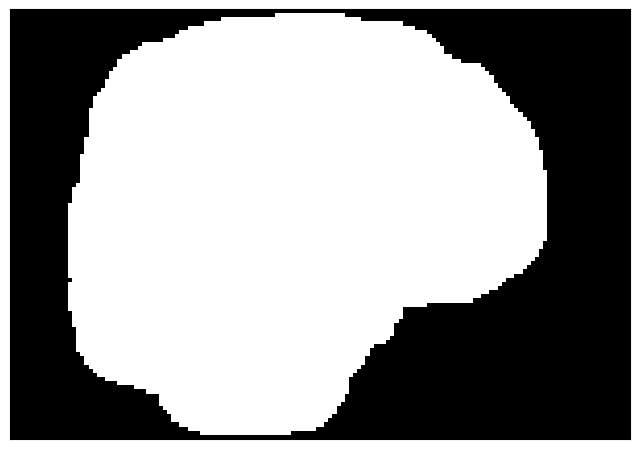

'/home/weberam2/Dropbox/AssistantProf_BCCHRI/Projects/Gavin_CSVO2/Quarto_Chisep_CSVO2_Manuscript/images/DilatedMask.png'

In [16]:

fourD_slice_cut = [slice(60, 190), slice(50, 200), slice(None), 1]
nii_gz_relpath = 'QSM_SSS/calc_chi/sub-AMWCER18/STISuite_Last3Echos/chi_dil7_echo5.nii.gz'
nii_gz_path = basepath + nii_gz_relpath

chidil_path="ChiDilated.png"
out_path=figpath + chidil_path

plot_and_save_nifti_slice(nii_gz_path, fourD_slice_cut, single_slice_cut, figsize, out_path, cmap)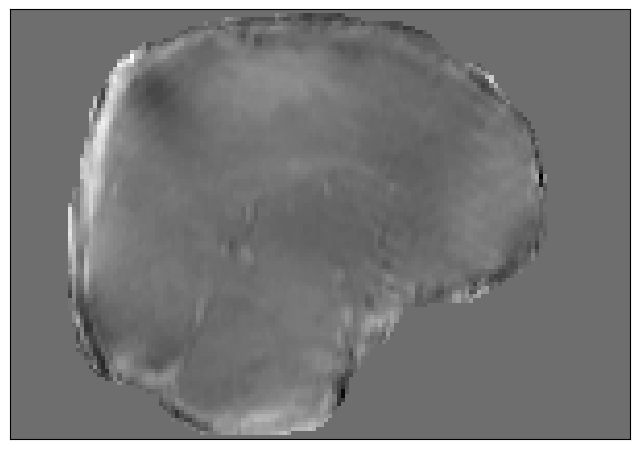

'/home/weberam2/Dropbox/AssistantProf_BCCHRI/Projects/Gavin_CSVO2/Quarto_Chisep_CSVO2_Manuscript/images/ChiDilated.png'

In [17]:

colors = ['black', 'red']
custom_cmap = ListedColormap(colors)

nii_gz_relpath = 'QSM_SSS/calc_chi/sub-AMWCER18/STISuite_Last3Echos/sss_dil7_echo5_mask.nii.gz'
nii_gz_path = basepath + nii_gz_relpath

sssmask_path="SSSMask.png"
out_path=figpath + sssmask_path

plot_and_save_nifti_slice(nii_gz_path, slice_cut, single_slice_cut, figsize, out_path, custom_cmap)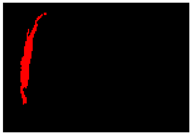

'/home/weberam2/Dropbox/AssistantProf_BCCHRI/Projects/Gavin_CSVO2/Quarto_Chisep_CSVO2_Manuscript/images/SSSMask.png'

In [18]:

nii_gz_path=basepath+'QSM_SSS/calc_chi/sub-AMWCER18/STISuite_Last3Echos/sss_dil7_echo5_mask.nii.gz'

# Load the NIfTI image
nii_img = nib.load(nii_gz_path)
nii_data = nii_img.get_fdata()

# Extract a single slice
subregion_data = nii_data[slice_cut[0], slice_cut[1], slice_cut[2]]
single_slice_data = subregion_data[single_slice_cut]

# Create a new figure with the specified figsize
plt.figure(figsize=figsize)

colors = ['black', 'red']
custom_cmap = ListedColormap(colors)

# Display the single slice with the specified colormap
plt.imshow(single_slice_data.T, cmap=custom_cmap, origin='lower')

nii_gz_path=basepath+'QSM_SSS/calc_chi/sub-AMWCER18/STISuite_Last3Echos/mag_echo5_sqr_brain_mask.nii.gz'

# Load the NIfTI image
nii_img = nib.load(nii_gz_path)
nii_data = nii_img.get_fdata()

subregion_data = nii_data[slice_cut[0], slice_cut[1], slice_cut[2]]

# Extract a single slice
single_slice_data2 = subregion_data[single_slice_cut]
mycmap = plt.cm.gray
mycmap.set_bad(alpha=0)
plt.imshow(single_slice_data2.T, cmap='gray', alpha=single_slice_data2.T, origin='lower', interpolation='none')

# Remove x-axis and y-axis ticks
plt.xticks([])
plt.yticks([])

finalmask_name="finalmask.png"
finalmask_path=figpath+finalmask_name
# Save the plot as a PNG file
plt.savefig(finalmask_path, dpi=300, bbox_inches="tight", pad_inches=0)

# Show the plot (optional)
plt.show()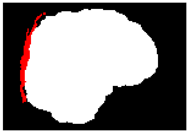

In [19]:

def resize_image_to_png(original_path, resize_percent, output_png_name):
    """
    Resize an image file and save it as a PNG file.

    Parameters:
    - sssmask_path (str): Path to the input image file.
    - resize_percent (float): Percentage by which to resize the image (e.g., 30 for 30%).
    - output_png_name (str): Desired name for the output PNG file (without the file extension).

    Returns:
    - str: Path to the saved PNG file.
    """
    # Load the image using Pillow
    img = Image.open(original_path)

    # Get the original width and height
    original_width, original_height = img.size

    # Calculate the new dimensions based on the percentage
    new_width = int(original_width * (resize_percent / 100))
    new_height = int(original_height * (resize_percent / 100))

    # Resize the image
    resized_img = img.resize((new_width, new_height))

    # Set the output file path for the resized image
    output_png_path = f"{output_png_name}.png"

    # Save the resized image as a PNG file
    resized_img.save(output_png_path)

    # Return the path to the saved PNG file
    return output_png_path

In [20]:

# Create a new graph
graph = graphviz.Graph(engine='neato')

# Add nodes with text and images
#graph.node('A', 'NifTI image file', shape='box', pos='0,0!')

resized_mag5_path = resize_image_to_png(figpath + magechofive_path, 30, figpath + "initialmag5_resized")
node_a_label = f'<<TABLE BORDER="0" CELLBORDER="0" CELLPADDING="1" CELLSPACING="0"><TR><TD><IMG SRC="{resized_mag5_path}" /></TD></TR><TR><TD ALIGN="CENTER">SWI magnitude, 5th echo</TD></TR></TABLE>>'
graph.node('A', label=node_a_label, shape='none', pos='0,0!')

graph.node('B', 'Create initial \nbrain mask', shape='ellipse', pos='2.5,0!')
graph.node('1', f'<<b>1</b>>', shape='none', pos='1.5,.3!')

resized_mask_path = resize_image_to_png(figpath + initialmask_path, 30, figpath + "initialmask_resized")
node_c_label = f'<<TABLE BORDER="0" CELLBORDER="0" CELLPADDING="1" CELLSPACING="0"><TR><TD><IMG SRC="{resized_mask_path}" /></TD></TR><TR><TD ALIGN="CENTER">Brain mask</TD></TR></TABLE>>'
graph.node('C', label=node_c_label, shape='none', pos='5,0!')

graph.node('D', 'Dilate', shape='ellipse', pos='6.7,0!')
graph.node('2', f'<<b>2</b>>', shape='none', pos='6.3,.3!')

dilmaskresized_image_path = resize_image_to_png(figpath + dilatedmask_path, 30, figpath + "dilmask_resized")
node_e_label = f'<<TABLE BORDER="0" CELLBORDER="0" CELLPADDING="1" CELLSPACING="0"><TR><TD><IMG SRC="{dilmaskresized_image_path}"/></TD></TR><TR><TD ALIGN="CENTER">Dilated brain mask</TD></TR></TABLE>>'
graph.node('E', label=node_e_label, shape='none', pos='8.5,0!')

graph.node('F', 'Calculate QSM with \ndilated mask', shape='ellipse', pos='8.5,-1.7!')
graph.node('3', f'<<b>3</b>>', shape='none', pos='7.3,-1.3!')

dilchiresized_image_path = resize_image_to_png(figpath + chidil_path, 30, figpath + 'dilchi_resized')
node_e_label = f'<<TABLE BORDER="0" CELLBORDER="0" CELLPADDING="1" CELLSPACING="0"><TR><TD><IMG SRC="{dilchiresized_image_path}"/></TD></TR><TR><TD ALIGN="CENTER">Dilated QSM image</TD></TR></TABLE>>'
graph.node('G', label=node_e_label, shape='none', pos='8.5,-3.4!')

graph.node('H', 'SSS segmentation',  shape='ellipse', pos='8.5,-5!')
graph.node('4', f'<<b>4</b>>', shape='none', pos='7.3,-4.75!')

sssmaskresized_image_path = resize_image_to_png(figpath + sssmask_path, 30, figpath + 'sssmask_resized')
node_i_label = f'<<TABLE BORDER="0" CELLBORDER="0" CELLPADDING="1" CELLSPACING="0"><TR><TD><IMG SRC="{sssmaskresized_image_path}"/></TD></TR><TR><TD ALIGN="CENTER">SSS mask</TD></TR></TABLE>>'
graph.node('I', label=node_i_label, shape='none', pos='5,-5!')

graph.node('J', 'Combine masks',  shape='ellipse', pos='5,-2.5!')
graph.node('5', f'<<b>5</b>>', shape='none', pos='4.2,-2.2!')

finalmaskresized_image_path = resize_image_to_png(figpath + finalmask_name, 30, figpath + 'finalmask_resized')
node_k_label = f'<<TABLE BORDER="0" CELLBORDER="0" CELLPADDING="1" CELLSPACING="0"><TR><TD><IMG SRC="{finalmaskresized_image_path}"/></TD></TR><TR><TD ALIGN="CENTER">Final mask with SSS</TD></TR></TABLE>>'
graph.node('K', label=node_k_label, shape='none', pos='2,-2.5!')

# Add edges between nodes
graph.edge('A', 'B', label='', constraint='false')
graph.edge('B', 'C', dir='forward', label='', constraint='false')
graph.edge('C', 'D', label='', constraint='false')
graph.edge('D', 'E', dir='forward', label='', constraint='false')
graph.edge('E', 'F',  label='', constraint='false')
graph.edge('F', 'G', dir='forward', label='', constraint='false')
graph.edge('G', 'H',  label='', constraint='false')
graph.edge('C', 'J',  label='', constraint='false')
graph.edge('I', 'J',  label='', constraint='false')
graph.edge('H', 'I', dir='forward', label='', constraint='false')
graph.edge('J', 'K', dir='forward', label='', constraint='false')

# Attributes
graph.attr(dpi='300', bgcolor='white', forcelabels='true')

# Render the graph
graph.render(figpath + 'example_graph', format='png', engine='neato', cleanup=True)

from IPython.display import Image as Ipmage
from IPython.display import display
from io import BytesIO

# Render the graph to a BytesIO object
png_bytes = graph.pipe(format='png')

# Display the graph using IPython.display
display(Ipmage(png_bytes))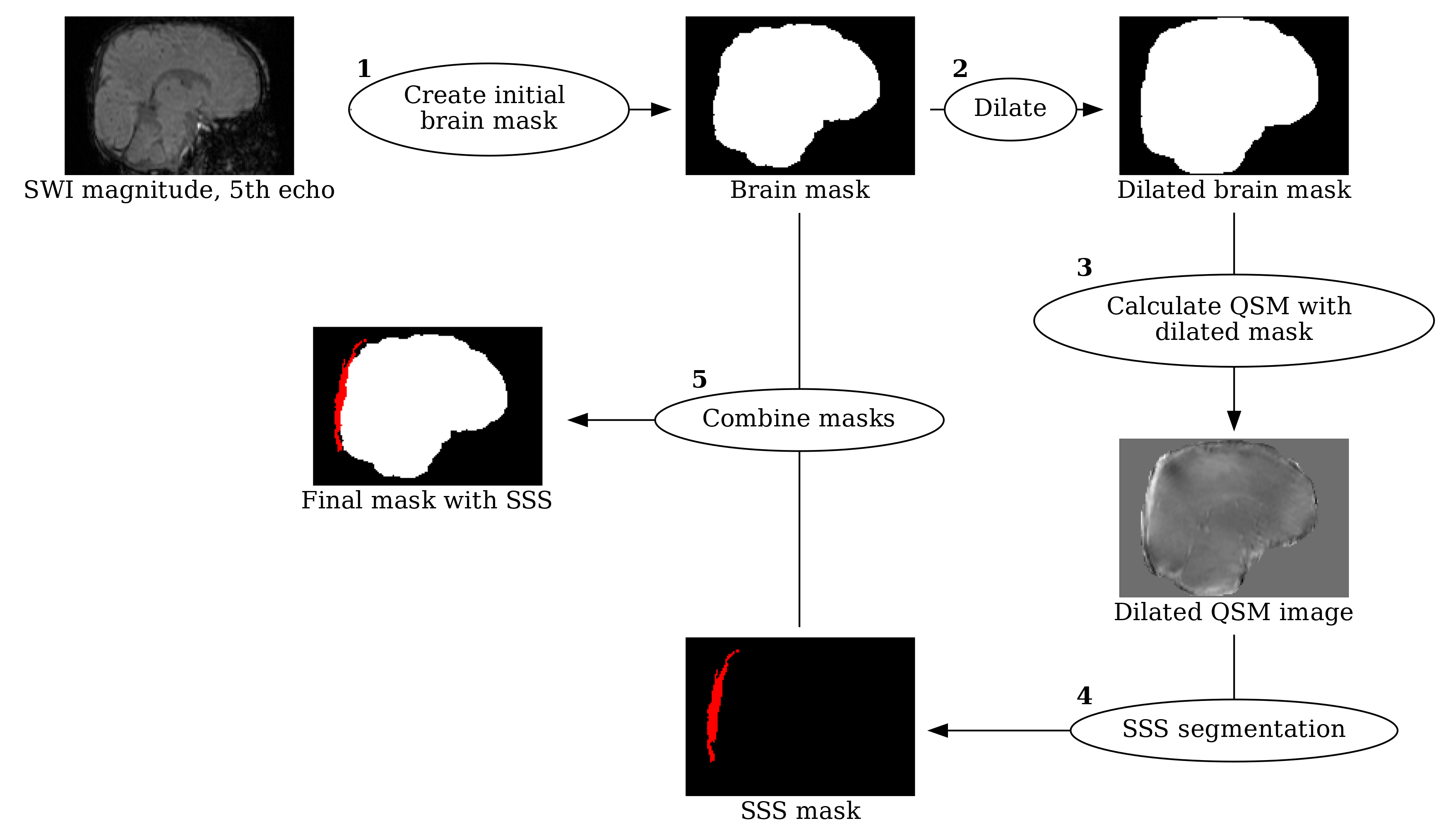

Figure 2: Pipeline for generating subject-specific brain masks that include the superior sagittal sinus (SSS). Initial steps involved (1) creating brain a mask from the magnitude of the fifth echo of the susceptibility weighted scan. Subsequently, the brain mask is dilated and then (2) utilized in conjunction with a quantitative susceptibility mapping (QSM) script to generate a preliminary QSM image. Further refinement involved (3) segmenting the SSS from the QSM image manually to create a tissue mask of the SSS region. Finally, (4) the vascular mask of the SSS is integrated with the initial brain mask, forming the comprehensive brain mask essential for obtaining susceptibility data that includes the SSS.

In [23]:

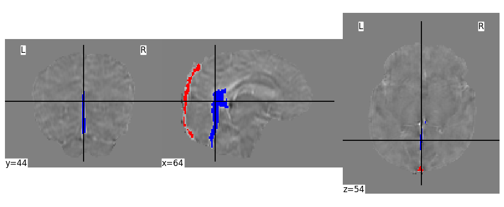
cut_coords_masks = (64,44,54)

sss_relpath = 'QSM_SSS/calc_chi/star_fsl/18/star_fsl_SSSmask.nii.gz'
sss_path = basepath + sss_relpath

ccv_relpath = 'QSM_SSS/calc_chi/star_fsl/18/star_fsl_intveinmask.nii.gz'
ccv_path = basepath + ccv_relpath

sssmask = apply_slice_cut_to_nifti(sss_path, slice_cut)
ccvmask = apply_slice_cut_to_nifti(ccv_path, slice_cut)

# Set the number of rows and columns for the subplot grid

#figsize=(10, 12)
#fig = plt.figure(figsize=figsize)

vmin, vmax = np.percentile(mag.get_fdata(), (2, 99.9))


display = plotting.plot_anat(
    anat_img=qsm,
    black_bg=False,
    draw_cross=True,
    vmin=-0.2, vmax=0.2,
    annotate=True,
    colorbar=False,
    cut_coords=cut_coords_masks,
    figure=plt.figure(figsize=(10, 4))
    #display_mode="mosaic"
)

redcolors = ['red']
custom_cmapred = ListedColormap(redcolors)
bluecolors = ['blue']
custom_cmapblue = ListedColormap(bluecolors)

display.add_overlay(sssmask, cmap=custom_cmapred)
display.add_overlay(ccvmask, cmap=custom_cmapblue)

plt.savefig(figpath + "SampleMasks.png", dpi=300, bbox_inches="tight")

plt.show()

Figure 3: Sample venous masks. A sample superior sagittal sinus (red) and central cerebral vein mask (blue) displayed in coronal, sagittal, and axial view. The QSM image is used as the underlay. y, x and z values represent the slice number in each plane (coronal, sagittal, and axial, respectively).